Gears Hammer of Dawn

Making a massive laser beam that’s coming from the sky feel impactful can’t be done by simply slapping some decals onto the ground and calling it a day like we would do for bullets or other small projectiles.

In this tutorial you’ll learn how to combine models, shaders, particles and post-processing in order to achieve a visual effect worthy of the Hammer of Dawn.

This tutorial is aimed towards beginners, so even without prior shader knowledge it should be easy to follow the step-by-step instructions. If you are more experienced and just looking for details, you should be able to easily identify the important passages and jump to them.

• 1 Effect Analysis
• 2 Model Setup
• 3 Unity Project
• 4 Getting Started
• 5 Ground Shader
• 6 Beam Shader
• 7 Finishing Touches

Effect Analysis

This time around, the tutorial wasn’t inspired by an ingame effect, but rather by the viz dev work of Klemen Lozar on Gears 5. He recently shared a bunch of it via twitter (@klemen_lozar), if you haven’t checked his account out already make sure to head over there and do so, there’s a lot of awesome stuff! For this tutorial, we’ll take a closer look at the Hammer of Dawn.

I did a lot of VFX viz dev on #Gears5 before leaving, got permission to post some of my favorite bits! Here I'm trying to show the awesome power of the Hammer Of Dawn, all animation is procedural using vertex shader techniques I already talked about #gamedev #realtimevfx #UE4 pic.twitter.com/tA9naGOzbk

— Klemen (@klemen_lozar) April 28, 2020

Let’s focus on the specific parts that make up the final effect. It’s tough to properly see the details of everything in fast-paced video, so let’s pause the video at 5 different points in time and take a closer look.

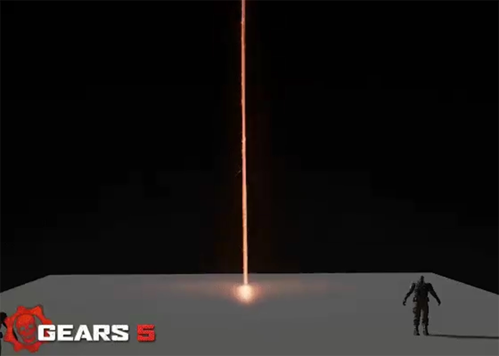
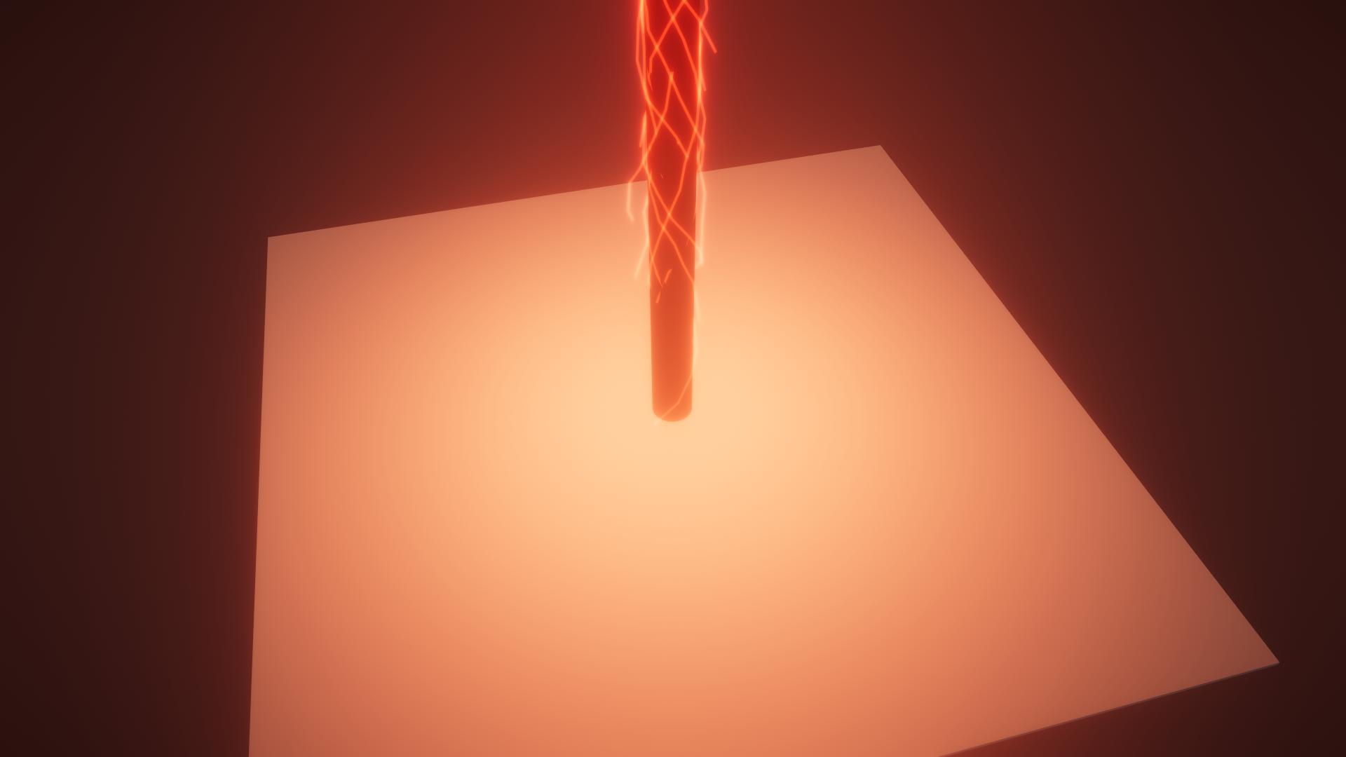
At the start of the effect’s sequence the laser beam starts growing in diameter over time. It emits light onto the surrounding area, which we’ll implement using a point light towards the end of the beam, as well as emission in combination with post-processing. Note that the beam isn’t quite straight; in motion you can see it wiggle slightly. Since the frequency of the wiggle is high the beam appears to be a bit more unstable, which adds to the final effect. One last thing you can see is the lightning particles around the beam. With the increasing size of the beam those particles also cover a wider cylinder, we’ll take a closer look at them in a later frame.

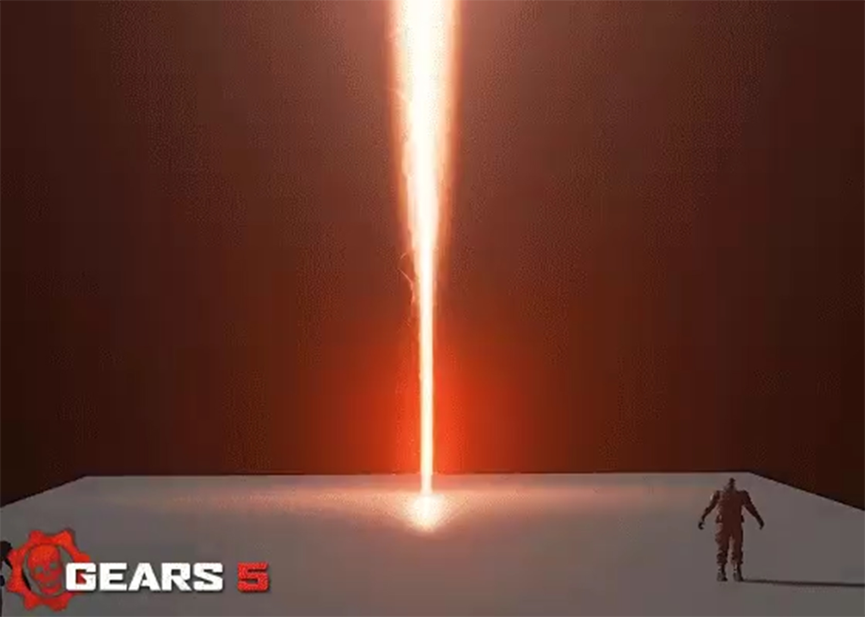
The ground in the next frame is still unchanged, the obvious point of interest is the shape of the beam. At some point the beam increases drastically in diameter, which, combined with the speed at which this broadening race towards the ground, results in this feel of an intense impact. You can see some of the previous mentioned lighting particles more clearly around the beam.

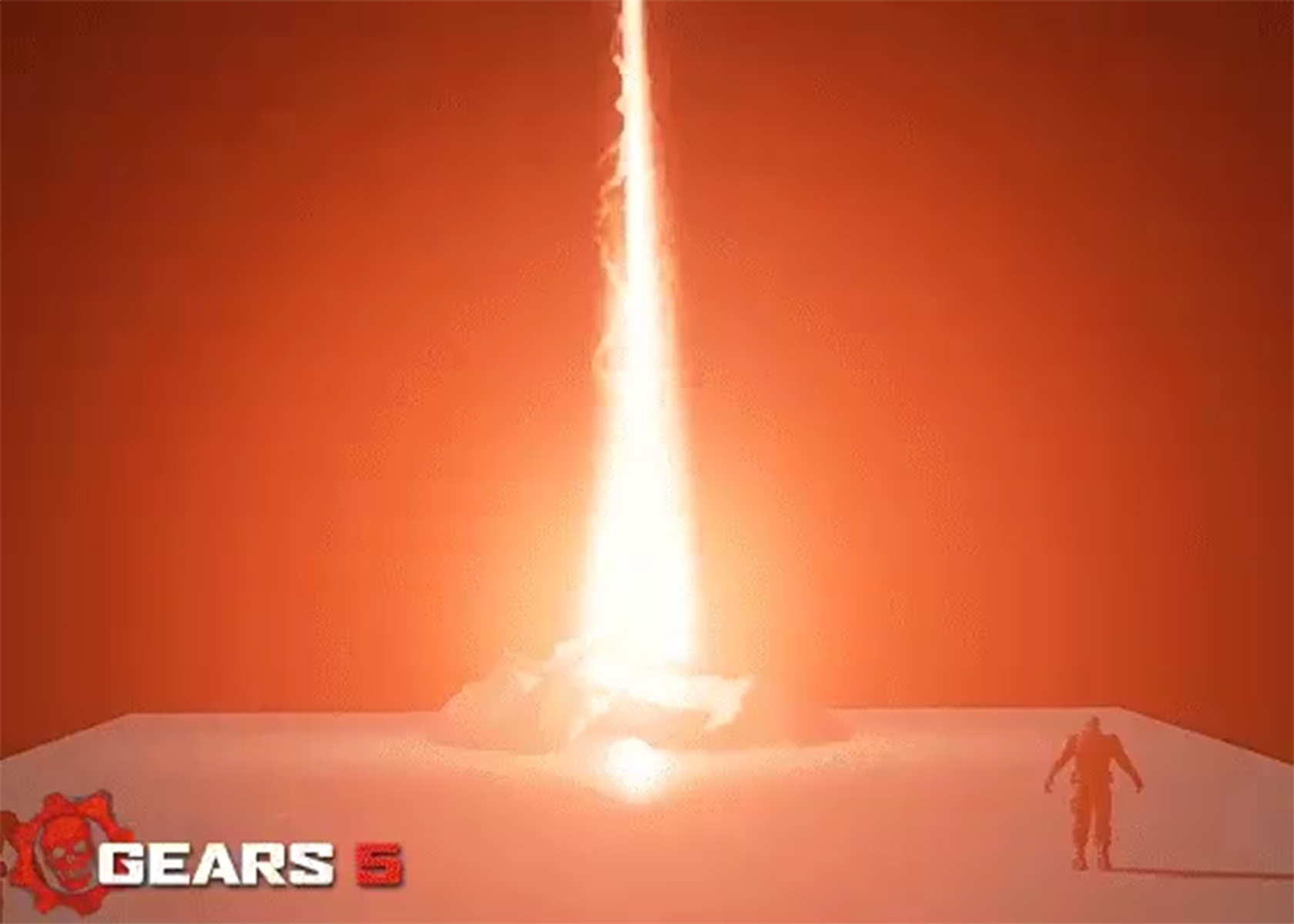
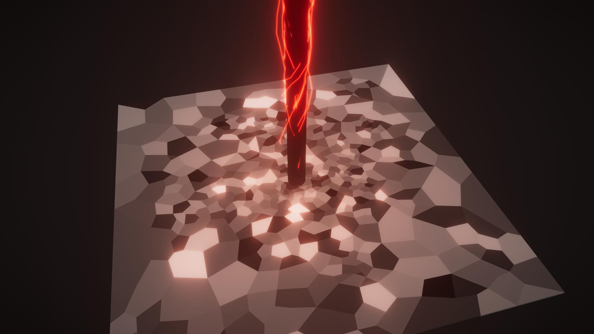
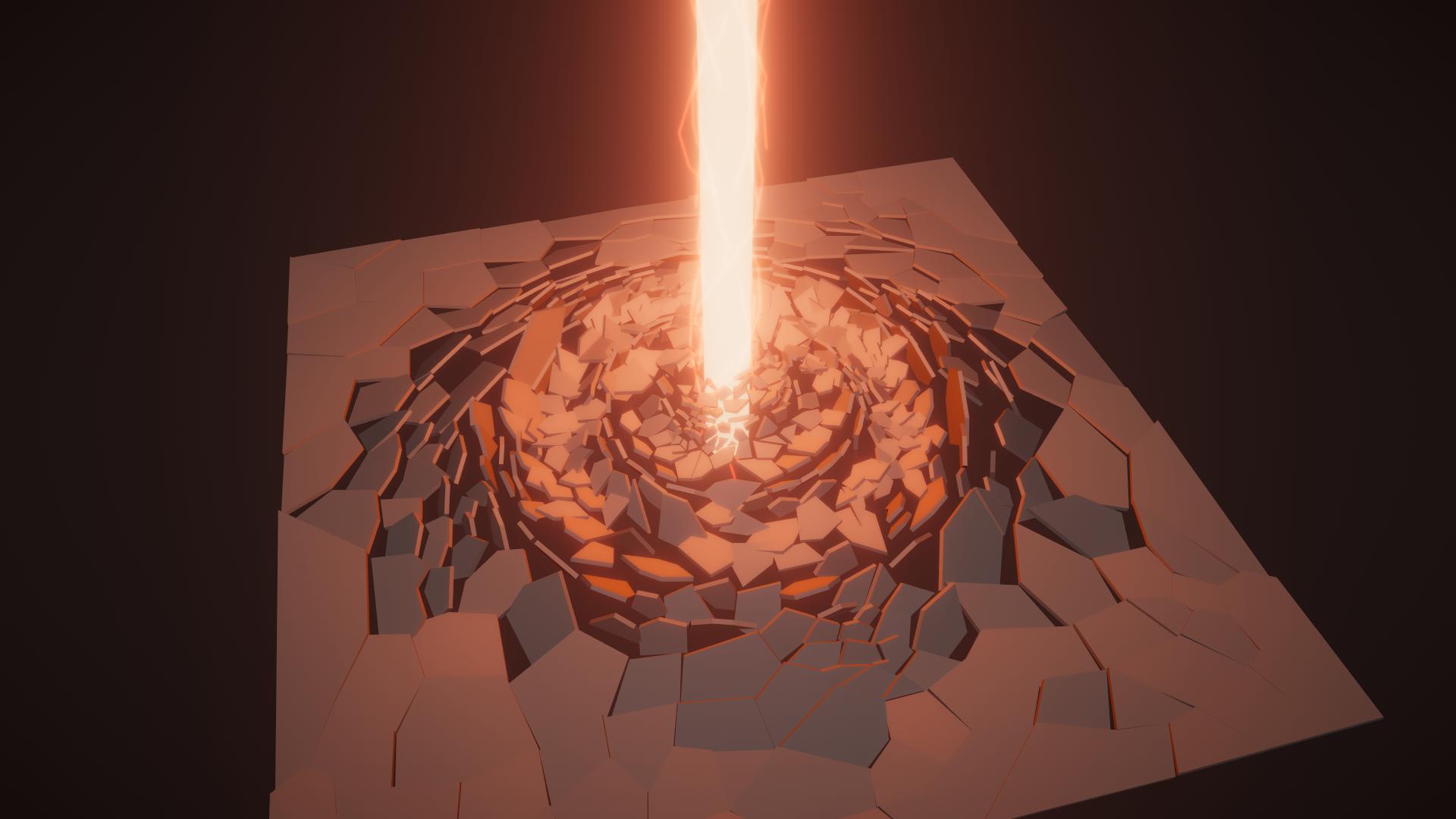
This is the moment of the impact. The ground starts to burst open and the light’s intensity increases a lot. Even though it is difficult to distinguish the lightning particles from the beam due to the high emission, you can see their structure more clearly in this frame. They appear to be wrapping around the beam, while still having this randomized, high frequent noise that determines their shape.

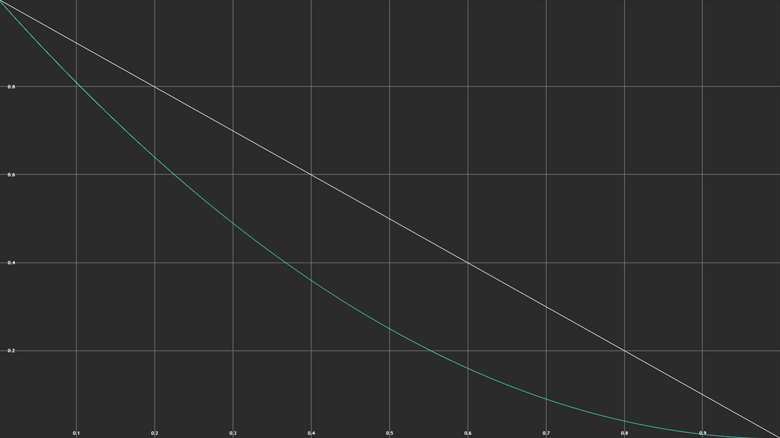
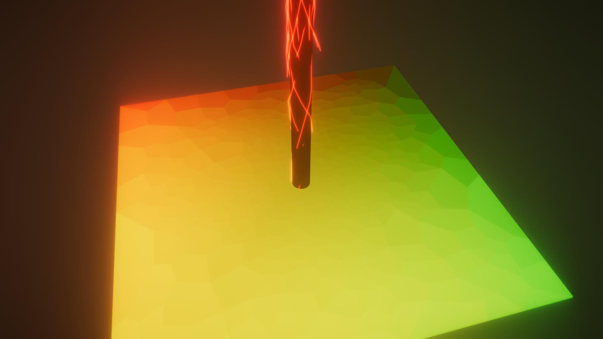
Except for some wiggling and randomized particles, the beam doesn’t really change anymore from this point. Let’s focus on the ground instead. The fragments burst into the air, the closer they are to the beam the further up they go. However, the height of the fragment doesn’t scale linearly with the distance to the beam; we can clearly see an exponential decay of this curve on the left side of the beam in this frame.

While moving upwards, the fragment also rotate away from the centre. Neighbouring fragments aren’t placed on the same height or rotate exactly by the same angle, indicating some noise value being present here to break up the monotony.

You can clearly see the exponential decay function for the height of the fragment in this one. In addition to the height offset, the fragments also get pushed away from the centre the higher they are. Gravity is somewhat simulated, meaning the fragments slow down when they are reaching their highest position and slowly begin to fall again.

What we can’t see in those 5 frames are the marks left by the beam on the ground underneath the cracked surface. You can clearly see this effect towards the end of the video. In order to keep this tutorial’s length somewhat reasonable we won’t implement that part, instead we’ll add some dust particles to fill the gaps and hide the end of the beam.

With all of that out of the way, let’s get started. I prepared a template project, which you can find on GitHub.

Template Project

It contains the Unity project with all the necessary resources you need to follow this tutorial. Since the model and project setup is quite specific to this effect, I’ll go over it in the next two chapters so you can understand the details. If you just want to get into the shaders, you can skip those chapters.

Model Setup

The models for this tutorial were created in Blender and exported as .fbx files to make sure everyone can import them into Unity, even without having Blender installed on their computer. This causes some issues with the coordinate system of the model, as the up vector in Blender (z axis) isn’t the same as the up vector in Unity (y axis). We’ll have to address this in the scene setup and the shaders later. This is not a modelling tutorial; this chapter should simply give you an idea about the procedure so you can adapt it if you need to.

Both models are part of the template project, you can skip this chapter if you are not interested in the model creation.

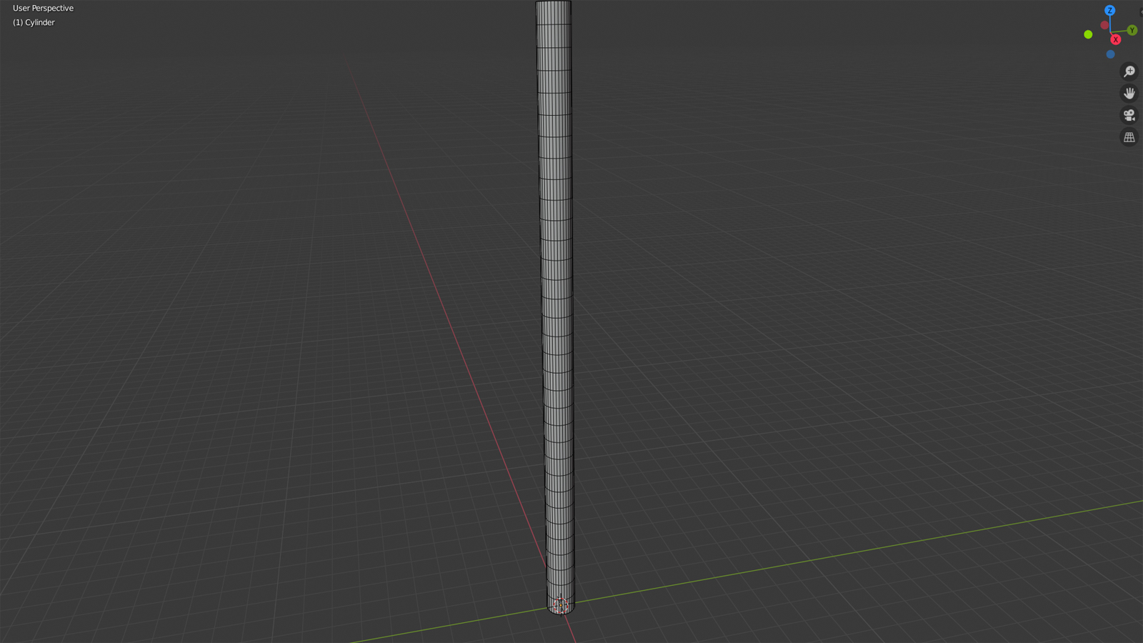
Let’s start with the beam model as it’s straight forward. I just added a cylinder to blender, scaled it along the z axis and added additional ring cuts to increase the vertex count.

The ground is a bit more complicated. I started with a plane and created the basic shapes of the fragments. There’s probably an amazing way to do this procedurally, but I’m not a 3D-artist and my Blender knowledge only goes so far.

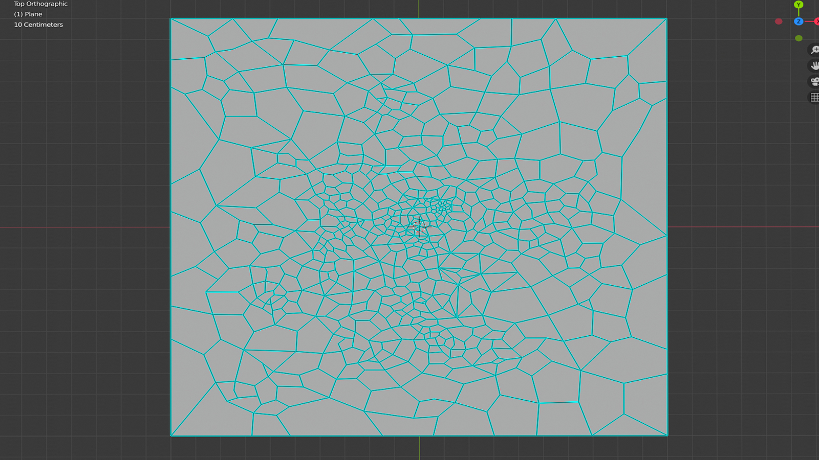
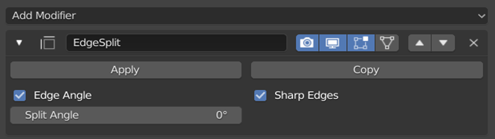
I added an edge split modifier to the model in order to split the fragments from each other. Since they are on a plane, the angel needs to be 0. After applying the modifier, we can move each fragment around individually.

In our vertex shader, we need to know for each vertex which fragment it is a part of. We can simply store the position of the fragment’s centre in the UV coordinate of each of its vertices. In order to do this in blender without custom scripts, we start by creating UV coordinates from projection.

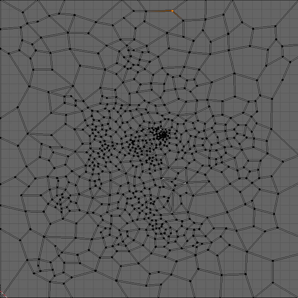
Afterwards, we can select each fragment individually in the UV editor and set its scale to 0. This gives us the wanted result of each vertex having its fragment’s centre stored in its UV coordinates.

The only thing left is to extrude the plane to give some thickness to the fragments. With that out of the way we can focus on the Unity project, so let’s take a look at the setup of the template project next.

Unity Project

By now, you should have downloaded the template project from GitHub. Since this is a shader tutorial, the bulk of the (non-shader) work in the scene is already prepared. If you are not interested in the project setup you can skip this part of the tutorial and jump to the next chapter where we’ll start to implement the shaders.

Open the “HammerOfDawn” scene placed in the root asset folder and press play. If everything works as intended, you should already see the following sequence:

As you can see, the particle effects, the lighting, the post-processing and the camera controls are all set up and already work. Let’s start our introduction with the basic structure of the scene.

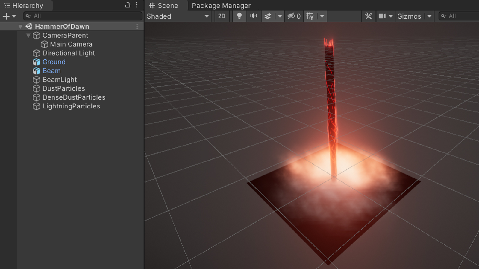
The “CameraParent” is used for orbiting the camera around the centre of the scene. It also holds the “SeqenceController.cs” script responsible for controlling the different components of the effect. The “MainCamera” is a child of this object which is easier for implementing camera shake and separating it from the orbital movement. We are using the “Post-Processing V2” package for post-processing, which requires having a Post-Process Layer and Volume.

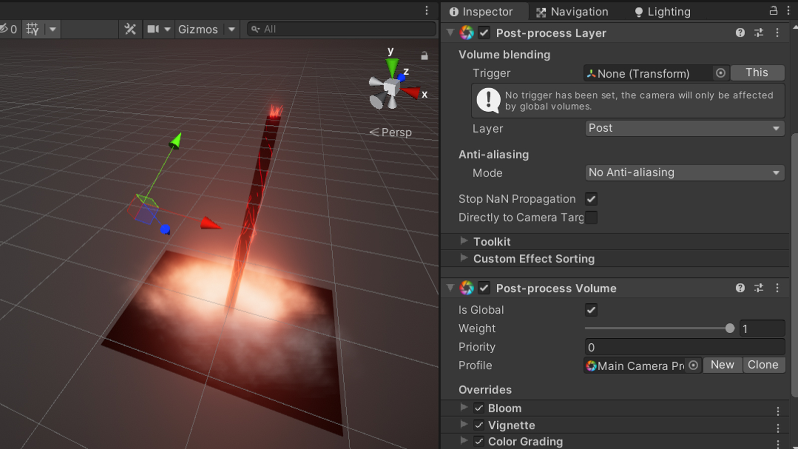
Since we are using MSAA, we don’t need post-processing based anti-aliasing. Our volume is global and contains bloom, a slight vignette and colour grading. We are using the linear colour space for the HDR colour grading to work properly.

The “DirectionalLight” in the scene is there for basic ambient lighting. We want the scene to be dark so the focus is more on the beam and the added bloom looks better, but we want to see at least the contours of our objects.

The “Ground” and “Beam” objects are, well, the objects for the ground and the beam (duh…). There are two aspects of interest regarding those two. First, the beam’s mesh renderer is set up to not cast or receive shadows. It is a highly emissive object and every shadow on it or behind it would look kind of weird. Second, you might have realized during the model setup and here that our ground is just a single model. You might have wondered why we go through all this trouble of baking fragment centres into the UV coordinates and not just have individual objects for each fragment. The reason for this is to optimize the performance of the effect, to be precise we want to reduce the amount of draw calls.

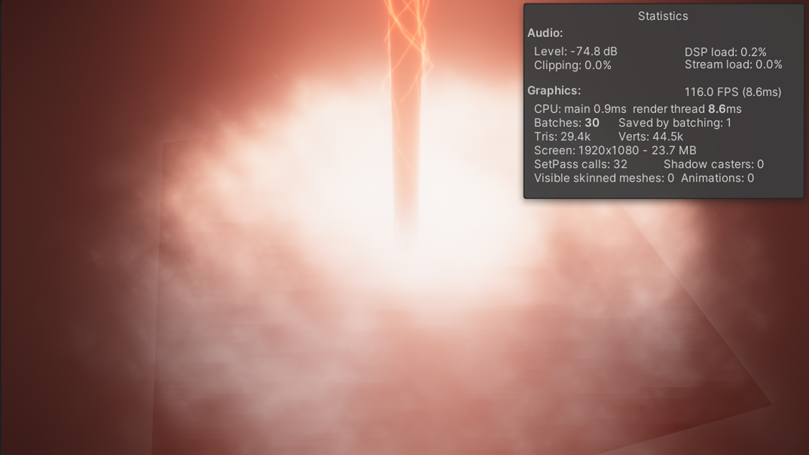
So instead of having 100 or more individual objects and thus a massive amount of draw calls we only have one and do some minor work in the shader to compensate for that. CPU bottlenecks due to high draw call counts are a regular reason for performance problems so knowing how to reduce them is a quite valuable skill to have.

Let’s get back to the scene structure. The next one on the list is the “BeamLight”, which is the point light we are using to add a bright emissive highlight on the environment around the beam.

The last three objects are the particle effects in the scene. The dust particles are used to fill holes in between the ground fragments upon impact, the dense particles are located around the end of the beam to hide that it just ends there (which would look ugly without the particles). The setup for the two dust particle systems is almost identical, except for the shape of the emission and the number of particles.

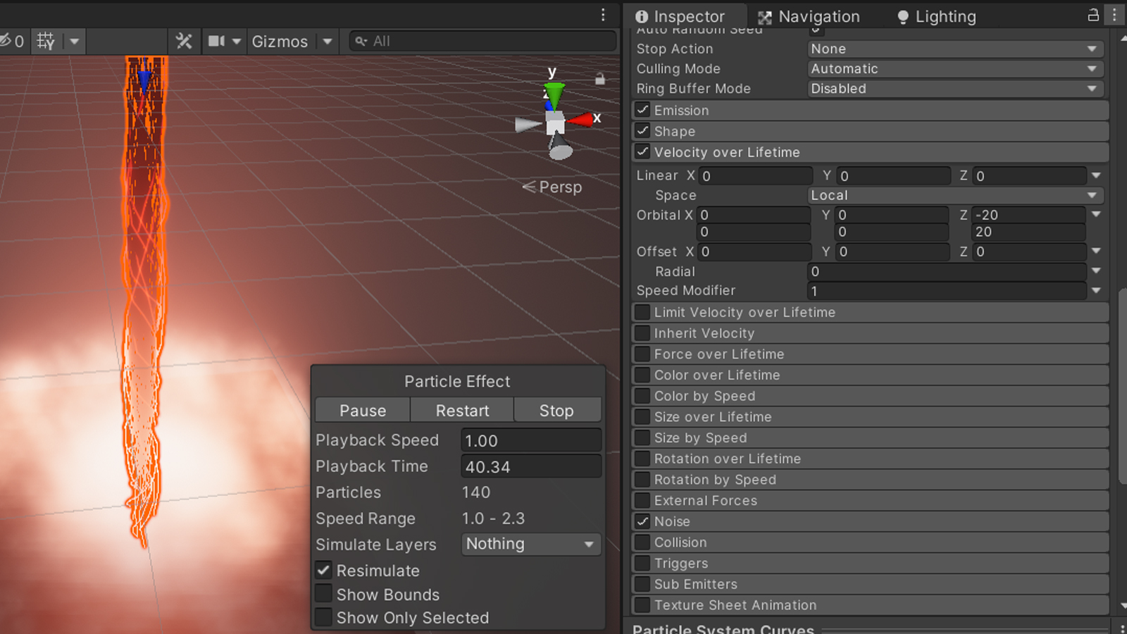
The lightning particles are more complicated than that and require a bit of an explanation as to how they work. The basic idea is to emit particles from the top of the beam and moving them along it. Instead of rendering the particles themselves, we only render their trail. We can add a high frequent noise to the particles to end up with a lightning-like shape.

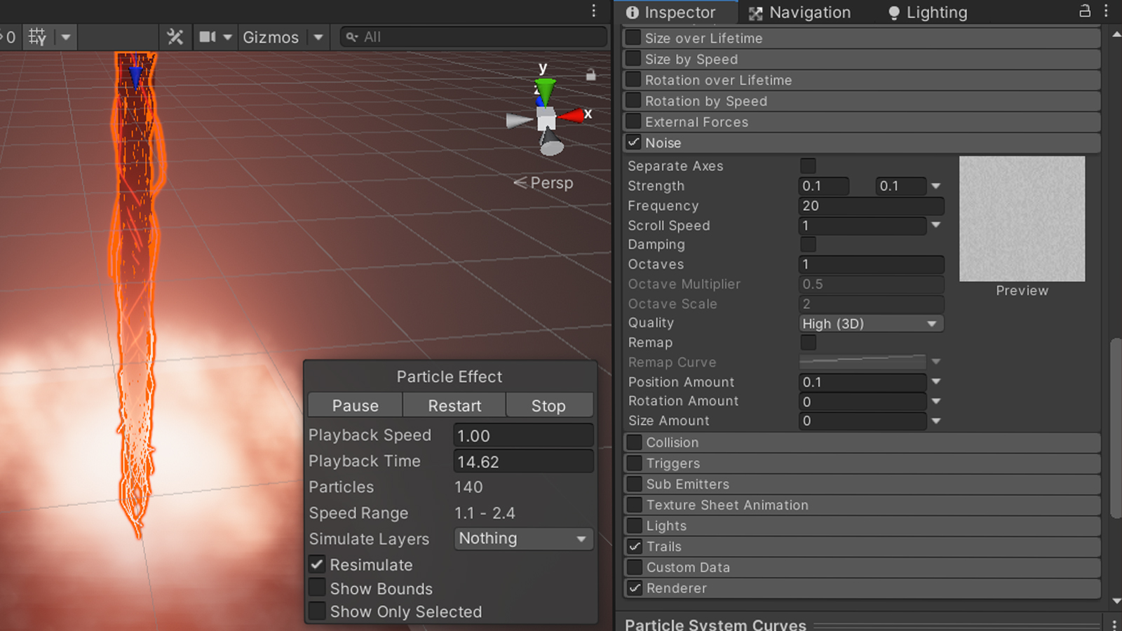
Due to the noise our lightning would end up all over the place, however we want to keep it close to the beam while still maintaining the noisy pattern. We can add a random orbital velocity to each a particle to make it circle the beam.

Alright, the last thing left we should look at is the sequence controller script. The first 45 lines of the script are just the public variables for all the objects in the scene, those should be self-explanatory so we can skip those.

private static readonly int Sequence = Shader.PropertyToID("_Sequence");
private static readonly int HeightMax = Shader.PropertyToID("_Sequence");

We are caching the shader property IDs to avoid having to do this lookup every frame. The variables inside the shaders that are controlling the sequence must have the same name (_Sequence) for the C# code to be able to set them.

SequenceVal += Time.deltaTime * 0.2f;
if (SequenceVal > 1.0f)
{
    SequenceVal = 0.0f;
    CameraTransform.localPosition = Vector3.zero;
}

In our update function, we first add the passed time (the time delta between the current and the previous frame) to our sequence value. Since it goes from 0 to 1, our sequence would be 1 second long if we add the unscaled time. I wanted it to take 5s, therefore I multiply the delta time with 0.2f. When the variable gets larger than 1, we simply reset it to restart the sequence. While we are here, we make sure to reset the camera shake by zeroing its position.

Transform localTransform;
(localTransform = transform).rotation = Quaternion.Euler(45.0f, SequenceVal * 120.0f + 15.0f, 0);
localTransform.position = -(localTransform.rotation * (Vector3.forward * 2.5f));

This is the code responsible for the orbiting camera. The rotation starts at 15 degrees and ends up at 135, the camera’s distance to the centre is 2.5f. If you want a faster or slower camera you can play around with the 120 degrees that are being multiplied with the sequence variable.

We follow two different code paths from here. The first part is the beam sequence, the second one is for the ground animation.

if (SequenceVal < 0.1f)
{
    GroundMat.SetFloat(Sequence, 0.01f - SequenceVal * 0.1f);

    BeamMat.SetFloat(HeightMax, Mathf.Pow(SequenceVal * 10.0f, 5.0f));

    LaserLight.intensity = SequenceVal * 8.0f;

    foreach (GameObject go in ParticleSystems)
        go.SetActive(false);

    LightningParticles.localScale = new Vector3(0.4f, 0.4f, 1.0f);
}

We start by slowly changing the sequence value in our ground shader from 0.01f to 0 which slightly cracks the ground and moves it downward a bit. We’ll see why when programming the shader. The next line exponentially changes the sequence value in the beam shader from 0 to 1. We increase the intensity of the point light to 8 and make sure our dust particles are deactivated. The last line adapts the scale of the lightning particles to be closer to the beam while its diameter is low.

else
{
    GroundMat.SetFloat(Sequence, SequenceVal * 1.09f - 0.09f);

    BeamMat.SetFloat(HeightMax, 1.0f);

    LaserLight.intensity = Mathf.Sin(Time.time * 30.0f) * 0.03f +
        Mathf.Sin(Time.time * 50.0f) * 0.03f +
        Mathf.Sin(Time.time * 7.0f) * 0.01f +
        0.8f;

    foreach (GameObject go in ParticleSystems)
    {
        go.SetActive(true);
    }

    LightningParticles.localScale = Vector3.one;

    CameraTransform.localPosition = Random.insideUnitSphere * 0.04f * (1.0f - SequenceVal);
}

In the second part of the sequence we change the ground’s sequence variable from 0.1f to 1 while keeping the beam’s variable at 1. We add some noise to the intensity of the point light by adding a variety of sinus waves on top of each other to make it look less regular. We activate the dust particles which spawn over time, reset the scale of the lightning particles and finally shake the camera by setting the position within a random sphere each frame.

Well, we are 2000 words in and still talking about the template project. I guess it is time to finally do what this tutorial is about and program some shaders! Sorry that it took so long but I promise that the result of this tutorial will be worth it.

Getting Started

Let’s start by thinking about what we want to do in our shaders. In both cases, we want to animate the vertices in the vertex function and output a single colour. Wouldn’t it be nice if we could simply use Unity’s lighting calculations and focus on just that? Well, turns out there’s a special kind of shader in Unity just for that. It’s called a surface shader; you might have heard of it before.

We start with the ground shader. Let’s open it and take a closer look at the structure of the shader, specifically at the differences between it and a standard vertex/fragment function setup. You can find the shaders in the "Shader" folder within the project's assets.

Shader "Lexdev/GearsHammer/Ground"

As with almost every shader in Unity, there is a ShaderLab program surrounding the actual code. This program starts with the name of the shader, you can change this to whatever you want but it might reset the variable values if you do so.

Properties
{

}

The property block is also still the same. It contains all the parameters that can be adjusted via the material’s inspector. We’ll add stuff to it in the next chapter.

SubShader
{
    CGPROGRAM
    ...
    ENDCG
}

The subshader block contains the actual shader code. For surface shaders, this needs to be CG instead of HLSL or GLSL. Their syntax is almost identical though so this shouldn’t bother you at all.

#pragma surface surf Standard vertex:vert

This line tells our compiler which function is our surface function. The default name is “surf”, and I left it like that for clarity. “Standard” identifies the lighting function that should be used for this shader, in our case the same lighting function as the one used for the Unity standard shader. The last parameter tells the compiler that we want to have a custom vertex function, and that it is called “vert”. Vertex functions are optional for surface shaders, as the compiler adds a default one for us.

struct Input
{
    float3 color;
};

The input struct is required by the surface function and it cannot be empty. In our case we don’t really need it I added a colour variable we can use for debugging later.

void vert(inout appdata_full v)
{

}

The vertex function receives and returns an appdata struct as an inout parameter. The appdata struct contains vertex information like position, normal, colour, UV and tangent. We can therefore simply modify values of this struct in our function without having to return it.

void surf (Input i, inout SurfaceOutputStandard o)
{
    
}

The surface function is simple. It is comparable to the output node of the shader graph, we simply set the shader properties and the lighting function (in our case the standard one) uses them to calculate the final colours. The shader properties are stored in the SurfaceOutputStandard struct; each entry has a value by default.

We only need to specifically set a couple of parameters, for the ground that is the colour, the metallic value and the smoothness.

void surf (Input i, inout SurfaceOutputStandard o)
{
+   o.Albedo = float3(1, 1, 1);
+   o.Metallic = 0;
+   o.Smoothness = 1;
}

You might have realized that those are the same values you would usually set in materials that are using the standard shader. For our case we can hardcode them, if you want to write a more adaptable shader you should add property variables for them.

The result looks like this, our ground is now white (well not really but its basic colour is) and the two lights in our scene influence it. Let’s move on to the interesting part, the vertex shader.

Ground Shader

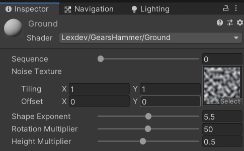
The ground shader is not as long and complicated as you might expect, however some basic knowledge of linear algebra is required. I’ll link to helpful resources whenever necessary so you can read up on some of the basics. For now, let’s start by adding a bunch of properties to our shader so we can control the effect from the inspector.

Properties
{
+   _Sequence("Sequence", Range(0,1)) = 0.0

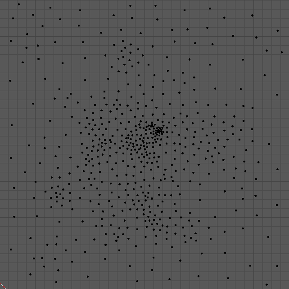
+   _Noise("Noise Texture", 2D) = "white" {}

+   _Exp("Shape Exponent", Range(1.0,10.0)) = 5.0
+   _Rot("Rotation Multiplier", Range(1.0,100.0)) = 50.0
+   _Height("Height Multiplier", Range(0.1,1.0)) = 0.5
}

The “_Sequence” variable is the one set by the C# controller script, so it is important that the name is written correctly. While the name for the other variables doesn’t really matter, it helps calling them the same way I do as they’ll automatically get the value I assigned to them in the final project.

A noise texture is used for some variation within the effect, without it, neighbouring fragments would always be at approximately the same position with almost the same orientation. Three more parameters control the shape and rotation of the fragment explosion. The shape exponent controls the previously mentioned exponential decay, the rotation multiplier the rotation of the fragments and the height multiplier the general height of the fragments.

+   float _Sequence;

+   sampler2D _Noise;

+   float _Exp;
+   float _Rot;
+   float _Height;

As always, we must add variables with the same name for each property to the actual shader code. Except for the noise texture, it’s all just simple float variables. With that, we can go to our vertex function.

void vert(inout appdata_full v)
{
+   float noise = tex2Dlod(_Noise, v.texcoord * 2.0f).r;
}

We start by calculating a noise value for our fragment. As we talked about earlier, v.texcoord (the UV of the vertex) stores its fragment’s position on the ground plane. I am multiplying it with 2 to get a higher frequent noise by using the fact that our texture is tileable and its wrap mode is set to repeat.

Textures can have multiple mip levels and vertex functions, unlike fragment function, do not know which mip level to choose when sampling the texture. That’s why we need to use tex2Dlod instead of tex2D, tex2Dlod requires an additional parameter that specifies which mip to use.

Let’s use the input struct to debug this noise value and see if it is per fragment as we intended.

+ void vert(inout appdata_full v, out Input i)
{
    float noise = tex2Dlod(_Noise, v.texcoord * 2.0f).r;

+   i.color = float3(noise, noise, noise);
}

void surf (Input i, inout SurfaceOutputStandard o)
{
+   o.Albedo = i.color;
    o.Metallic = 0;
    o.Smoothness = 1;
}

As you can see, all we must do is return an input struct from our vertex function with a colour set to our noise value and set it as colour in our SurfaceOutput struct. The result should look like this (I increased the directional light intensity so you can see it better):

Looks like everything works as intended! We have a noise value for each vertex that depends on the fragment it is a part of. You can also output the UV coordinates directly to see this:

void vert(inout appdata_full v, out Input i)
{
    float noise = tex2Dlod(_Noise, v.texcoord * 2.0f).r;

+   i.color = float3(v.texcoord.xy, 0);
}

We can see that our UVs range from (0,0) in one corner to (1,1) in the opposite one, just as we intended. Since we want to start our explosion at the centre, we need to calculate UV coordinates relative to it.

void vert(inout appdata_full v, out Input i)
{
    float noise = tex2Dlod(_Noise, v.texcoord * 2.0f).r;
+   float2 uvDir = v.texcoord.xy - 0.5f;

    i.color = float3(v.texcoord.xy, 0);
}

Let’s think about our sequence for a moment. What we are effectively doing is calculate a vertex position based on the “_Sequence” variable and a couple of parameters. For ease of use, the “_Sequence” variable ranges from 0 to 1, however this might not be the range of the explosion function we want to display. Through testing, I figured out that the actual range is -0.02f to 1.5f.

void vert(inout appdata_full v, out Input i)
{
    float noise = tex2Dlod(_Noise, v.texcoord * 2.0f).r;
    float2 uvDir = v.texcoord.xy - 0.5f;
+   float scaledSequence = _Sequence * 1.52f - 0.02f;

    i.color = float3(v.texcoord.xy, 0);
}

While those values might look a bit random, we’ll see later why they are what they are. For now, let’s create the basic shape of our explosion.

void vert(inout appdata_full v, out Input i)
{
    float noise = tex2Dlod(_Noise, v.texcoord * 2.0f).r;
    float2 uvDir = v.texcoord.xy - 0.5f;
    float scaledSequence = _Sequence * 1.52f - 0.02f;

+   float seqVal = pow(1.0f - (noise + 1.0f) * length(uvDir), _Exp) * scaledSequence;

    i.color = float3(v.texcoord.xy, 0);
}

Okay, quite a lot to unpack here. First, let’s focus on 1.0f – (noise + 1.0f) * length(uvDir). We want to calculate a value that decreases the further away from the centre we are while also adding some noise to the distance in order to break up the pattern a bit. This decrease shouldn’t be linear, but rather exponential, hence the pow() function enclosing it. Lastly, we must multiply it with our scaled sequence value since we want to scale this effect over time. If we debug this value, we can already see the effect we want:

void vert(inout appdata_full v, out Input i)
{
    float noise = tex2Dlod(_Noise, v.texcoord * 2.0f).r;
    float2 uvDir = v.texcoord.xy - 0.5f;
    float scaledSequence = _Sequence * 1.52f - 0.02f;

    float seqVal = pow(1.0f - (noise + 1.0f) * length(uvDir), _Exp) * scaledSequence;

+   i.color = float3(seqVal, seqVal, seqVal);
}

All that’s left for us to do is use this value to modify the height, position and rotation of the fragment and our ground is done! Let’s start with the height.

void vert(inout appdata_full v, out Input i)
{
    float noise = tex2Dlod(_Noise, v.texcoord * 2.0f).r;
    float2 uvDir = v.texcoord.xy - 0.5f;
    float scaledSequence = _Sequence * 1.52f - 0.02f;

    float seqVal = pow(1.0f - (noise + 1.0f) * length(uvDir), _Exp) * scaledSequence;

+   v.vertex.z += sin(seqVal * 2.0f) * (noise + 1.0f) * _Height;

    i.color = float3(seqVal, seqVal, seqVal);
}

The height calculations are the easiest of the three. The basic idea is to multiply our calculated sequence value with some noise and our height variable and add it to the height of the vertex (which is z in our case due to the blender coordinate system conversion). Let’s talk about the sinus in there. We want to somewhat simulate gravity towards the end of the sequence by having some of the fragment falling. Taking only the first part of a sinus wave gives us this behaviour. The result should look like this:

Let’s tackle horizontal movement next. Our fragments should move further away from the centre the higher they are, which means we can simply scale their position offset with our sequence value as well.

void vert(inout appdata_full v, out Input i)
{
    float noise = tex2Dlod(_Noise, v.texcoord * 2.0f).r;
    float2 uvDir = v.texcoord.xy - 0.5f;
    float scaledSequence = _Sequence * 1.52f - 0.02f;

    float seqVal = pow(1.0f - (noise + 1.0f) * length(uvDir), _Exp) * scaledSequence;

    v.vertex.z += sin(seqVal * 2.0f) * (noise + 1.0f) * _Height;
+   v.vertex.xy -= normalize(float2(v.texcoord.x, 1.0f - v.texcoord.y) - 0.5f) * seqVal * noise;

    i.color = float3(seqVal, seqVal, seqVal);
}

You might be wondering why we are calculating a new vector for the position relative to the centre instead of using the “uvDir” variable. The model is set up in a way that we must flip the y coordinate of the UV, which didn’t matter in our previous calculations where we only used the length of the vector. After this step, the effect should look like this:

Now, let’s talk about rotation. In order to rotate a vertex and its normal, we need two know three things: The point around which we want to rotate the object, the axis and the angle. I’ll show you the helper function we are writing for this first and discuss if afterwards, as I think it is easier to understand it that way.

+ void Rotate(inout float4 vertex, inout float3 normal, float3 center, float3 around, float angle)
+ {
+   float4x4 translation = float4x4(
+   1, 0, 0, center.x,
+   0, 1, 0, -center.y,
+   0, 0, 1, -center.z,
+   0, 0, 0, 1);
+   float4x4 translationT = float4x4(
+   1, 0, 0, -center.x,
+   0, 1, 0, center.y,
+   0, 0, 1, center.z,
+   0, 0, 0, 1);
+
+   around.x = -around.x;
+   around = normalize(around);
+   float s = sin(angle);
+   float c = cos(angle);
+   float ic = 1.0 - c;
+
+   float4x4 rotation = float4x4(
+   ic * around.x * around.x + c, ic * around.x * around.y - s * around.z, ic * around.z * around.x + s * around.y, 0.0,
+   ic * around.x * around.y + s * around.z, ic * around.y * around.y + c, ic * around.y * around.z - s * around.x, 0.0,
+   ic * around.z * around.x - s * around.y, ic * around.y * around.z + s * around.x, ic * around.z * around.z + c, 0.0,
+   0.0, 0.0, 0.0, 1.0);
+
+   vertex = mul(translationT, mul(rotation, mul(translation, vertex)));
+   normal = mul(translationT, mul(rotation, mul(translation, float4(normal, 0.0f)))).xyz;
+ }

While this function is a bit longer than the previous code snippets, the functionality is quite simple. We are creating a translation matrix for the centre point to move the vertex before rotating it and the inverse translation matrix for moving it back. We must flip the x axis due to the Blender Unity coordinate system shenanigans but other than that it’s simple as that.

After the two translation matrixes, we are calculating a bunch of values we regularly need in the rotation matrix, such as the sinus and cosinus of the angle. There is nothing special about the rotation matrix itself, just a regular rotation around an arbitrary axis.

When multiplying the matrices with the position and normal vectors, it is important that the order of the multiplications is correct. Other than that, it is just as straightforward as that.

void vert(inout appdata_full v, out Input i)
{
    float noise = tex2Dlod(_Noise, v.texcoord * 2.0f).r;
    float2 uvDir = v.texcoord.xy - 0.5f;
    float scaledSequence = _Sequence * 1.52f - 0.02f;

    float seqVal = pow(1.0f - (noise + 1.0f) * length(uvDir), _Exp) * scaledSequence;

+   Rotate(v.vertex, v.normal, float3(2.0f * uvDir, 0), cross(float3(uvDir, 0), float3(noise * 0.1f, 0, 1)), seqVal * _Rot);

    v.vertex.z += sin(seqVal * 2.0f) * (noise + 1.0f) * _Height;
    v.vertex.xy -= normalize(float2(v.texcoord.x, 1.0f - v.texcoord.y) - 0.5f) * seqVal * noise;

+   i.color = float3(1,1,1);
}

Let’s discuss the parameters of the function call. The first two parameters are the position and the normal vector which we get from the appdata struct. The third parameter is the position of the fragment centre around which we want to rotate. The ground object is 2x2 units large, so if we want to map UV coordinates (which are [0;1]) onto it we simply must multiply with 2.

The fourth parameter is the axis around which we rotate. This one isn’t quite as straight forward, as we want this axis to be orthogonal to the vector from the centre to the fragment’s position. If we do that, our fragment rotates away from the centre. We can calculate such an axis by doing a cross product between to vector from the centre to the position and the up vector. We slightly modify this up angle using our noise value to add some variation to the rotation. As for the angle, we simply use our sequence value so objects closer to the centre rotate more and multiply it with our rotation property to have more control over the rotation overall.

While we are here, we change the colour back to white to disable the debug output.

And with that we are done with the ground shader, next up is the one for them beam. Already looks quite nice doesn’t it? You should play around with the parameters and see if you can adapt the shader to your liking. Let’s keep going.

Beam Shader

If you recall the effect analysis section, there are two things we need to implement for the beam shader; the basic shape of the beam depending on the sequence value and some noise to make the beam appear less stable. If you open the beam shader, you’ll see that it’s the same basic framework as the ground shader. The Input struct is once again unused and can be used for debugging.

Let’s get the properties and the surface function out of the way first.

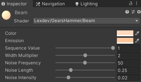
Properties
{
+   _Color("Color", Color) = (1,1,1,1)
+   _Emission("Emission", Color) = (1,1,1,1)

+   _Sequence("Sequence Value", Range(0,1)) = 0.1

+   _Width("Width Multiplier", Range(1,3)) = 2

+   _NoiseFrequency("Noise Frequency", Range(1,100)) = 50.0
+   _NoiseLength("Noise Length", Range(0.01,1.0)) = 0.25
+   _NoiseIntensity("Noise Intensity", Range(0,0.1)) = 0.02
}

“_Color” and “_Emission” are the basic colour of the beam and its emissive colour. “_Sequence” is the variable referenced by the C# controller script and fulfils the same purpose here, it controls the position in the effect’s sequence. The “_Width” property is just a general multiplier for the beam’s width to increase or decrease its diameter. The last three properties control different aspects of the noise function that wiggles the beam.

+   fixed4 _Color;
+   fixed4 _Emission;

+   float _Sequence;

+   float _Width;

+   float _NoiseFrequency;
+   float _NoiseLength;
+   float _NoiseIntensity;

Don’t forget to add variables for the properties to the cg code. Except for the colours, all our properties are float variables.

The surface function is as easy as before, all we must do is set the values of our SurfaceOutput struct.

void surf (Input IN, inout SurfaceOutputStandard o)
{
+   o.Albedo = _Color.rgb;
+   o.Emission = _Emission;
+   o.Metallic = 0;
+   o.Smoothness = 1;
}

Albedo, Metallic and Smoothness values work just as before, what’s new is the Emission variable. With it, we can make the beam glow in the colour we specify in our property, which works nicely with the bloom post processing.

While our beam is not quite done yet, at least it doesn’t look like a placeholder anymore.

Let’s shift our focus to the vertex function, we’ll do the shape of the beam first. As mentioned in the effect analysis, the beam consists of three parts. First, the part below the broadening is thin and slowly grows in diameter over time. Second, the broadening itself which has a radius in the form of a maximum of a sinus function. And Third, the part above the broadening which has a constant diameter and is the part visible for most oft the effect. We start by storing the beam’s height in a variable since we need it often.

void vert(inout appdata_full v)
{
+   float beamHeight = 20.0f;
}

This is highly specific to the model, we need this value to determine where our vertex is located on the beam’s cylinder (at the bottom, at the top, …).

void vert(inout appdata_full v)
{
    float beamHeight = 20.0f;

+   float scaledSeq = (1.0f - _Sequence) * 2.0f - 1.0f;
}

Our sequence value ranges from 0 to 1, and we want it to determine where our broad part is located on the beam. At the start of the sequence we want the broadening to be at the top of the beam, in the middle of the sequence it should be at the bottom, looking like it crashes into the ground. Afterwards, towards the end of the sequence, it should disappear and the whole beam should look like the part above the maximum, having a constant width and only some noise. We can simulate this by moving the broadening to a value of -1, which is underneath the ground and out of our view. In short, a sequence value of 0 should map to 1 and a sequence value of 1 to -1. The function above achieves just that, it inverts the value and scales the range.

void vert(inout appdata_full v)
{
    float beamHeight = 20.0f;

    float scaledSeq = (1.0f - _Sequence) * 2.0f - 1.0f;
+   float scaledSeqHeight = scaledSeq * beamHeight;
}

We multiply the scaled sequence value with our beam’s actual height so a sequence value of 0 is located at the top of the beam, a sequence value of -1 at the negative height of the beam.

void vert(inout appdata_full v)
{
    float beamHeight = 20.0f;

    float scaledSeq = (1.0f - _Sequence) * 2.0f - 1.0f;
    float scaledSeqHeight = scaledSeq * beamHeight;

+   float cosVal = cos(3.141f * (v.vertex.z / beamHeight - scaledSeq));

+   v.vertex.xy *= cosVal;
}

Let’s start modelling the broadening part of our function first. We start with a cosinus wave that is the length of two times our beam height. If we subtract the scaled sequence value, we shift the maximum to the position we want (at 1 if our sequence is 0, at -1 if it’s 1). We can multiply this cosinus value with our width in x and y direction to display it.

Currently the pattern is repeating infinitely, we now must calculate functions for the parts below and above the broadening and blend between the three functions. For blending we can use lerp and a smoothstep function.

void vert(inout appdata_full v)
{
    float beamHeight = 20.0f;

    float scaledSeq = (1.0f - _Sequence) * 2.0f - 1.0f;
    float scaledSeqHeight = scaledSeq * beamHeight;

    float cosVal = cos(3.141f * (v.vertex.z / beamHeight - scaledSeq));
+   float width = lerp(0.05f * (beamHeight - scaledSeqHeight + 0.5f), 
+                               cosVal, 
+                               pow(smoothstep(scaledSeqHeight - 8.0f, scaledSeqHeight, v.vertex.z), 0.1f));

+   v.vertex.xy *= width;
}

The 3 parameters of the lerp function are the function for below the maximum, our cosinus function for the maximum and the smoothstep function we are using to blend between them. Let’s go through them one by one. “0.05f * (beamHeight - scaledHeightMax + 0.5f)” describes a small beam that grows in diameter the closer our maximum position is to the bottom of the beam. Our cosinus variable is unchanged, the interesting part is the third parameter, the lerp value. A lerp value of 0 means the function returns the first parameter, a value of 1 returns the second parameter. The smoothstep function evaluates, whether our vertex position is lower than the current position of the broadening minus 8.0f, above the broadening or in between. It returns 0, 1 or a smooth blend between them respectively, leading to a smooth blend between the two first parameters of the lerp. The pow() function slightly changes the blend shape. If we use this value to modify the diameter of the beam, we can see that we properly modelled the bottom part.

void vert(inout appdata_full v)
{
    float beamHeight = 20.0f;

    float scaledSeq = (1.0f - _Sequence) * 2.0f - 1.0f;
    float scaledSeqHeight = scaledSeq * beamHeight;

    float cosVal = cos(3.141f * (v.vertex.z / beamHeight - scaledSeq));
    float width = lerp(0.05f * (beamHeight - scaledSeqHeight + 0.5f),
                                cosVal,
                                pow(smoothstep(scaledSeqHeight - 8.0f, scaledSeqHeight, v.vertex.z), 0.1f));

+   width = lerp(width,
+                0.4f,
+                smoothstep(scaledSeqHeight, scaledSeqHeight + 10.0f, v.vertex.z));

+   v.vertex.xy *= width * _Width;
}

Modelling the beam above the broadening is easier, as it just has a constant width. We blend a bit more slowly between the functions (over 10 units instead of 8) but other than that the behaviour is the same. While we are here, we multiply our “_Width” property with the final value to be able to modify it from the inspector.

One more line of code to do.

void vert(inout appdata_full v)
{
    float beamHeight = 20.0f;

    float scaledSeq = (1.0f - _Sequence) * 2.0f - 1.0f;
    float scaledSeqHeight = scaledSeq * beamHeight;

    float cosVal = cos(3.141f * (v.vertex.z / beamHeight - scaledSeq));
    float width = lerp(0.05f * (beamHeight - scaledSeqHeight + 0.5f),
                                cosVal,
                                pow(smoothstep(scaledSeqHeight - 8.0f, scaledSeqHeight, v.vertex.z), 0.1f));

    width = lerp(width,
                 0.4f,
                 smoothstep(scaledSeqHeight, scaledSeqHeight + 10.0f, v.vertex.z));

    v.vertex.xy *= width * _Width;

+   v.vertex.xy += sin(_Time.y * _NoiseFrequency + v.vertex.z * _NoiseLength) * _NoiseIntensity * _Sequence;
}

Adding some noise is simple. We add a sinus function over time and height of the vertex which we are scaling in various ways using our previously added properties. First, we can change the frequency of the sinus by multiplying the time with our frequency value. Second, we can change the physical length of the wave across the height of our beam by multiplying the vertex height with the length property. By multiplying with the intensity, we can change the extends of the sinus. Lastly, we multiply with the sequence value to increase the strength of the wiggle over time. As a result, we get this unstable beam effect we are looking for.

Finishing Touches

If you want to exactly replicate my results, here are the material properties I chose:

Make sure all objects in the scene and the controller script are enabled if you disabled them during debugging.

All Done!

That’s it! With all the stuff you just learned you can start creating awesome shader and particle effects for your next game. I’m really impressed that you worked through all of this! If you happened to run into any issues, you should check out the final version of the project.

Final Project

If you build something in the future that is based on this tutorial or the things you learned in it, make sure to share it via reddit or twitter and let me know, I'm always interested in seeing what you guys create. You can also use twitter to send me questions and suggest future topics. See you next time!